Same Start, Different Outcomes: What the Opportunity Atlas Shows About West Orange
Continuing in the spirit of telling data stories about my community, I was intrigued by the possibility of exploring how it shows up in one of my favorite data tools. I live in West Orange, and like a lot of people who study place and opportunity, I have spent more time than I'd like to admit clicking around the Opportunity Atlas exploring the differential outcomes in neighborhoods I’ve lived in over the course of my life. The Opportunity Atlas is the map Raj Chetty and his colleagues built from Census and federal tax records. For every census tract in the country, it estimates how the children who grew up there were doing as adults [1]. The idea for this examination came to me while working on a data tool about West Orange school performance, and I pulled our nine tracts as a thought exercise.
The Atlas asks a narrow question. Take children whose parents were at the 25th percentile of the national income distribution. That is the income level where roughly 25% of parents with kids the same age earn less and 75% earn more, roughly $27,000 a year. Follow those children into their early-to-mid 30s to see where they landed. The children in this data were born between 1978 and 1983, grew up in the 1980s and 1990s, and had their incomes measured in 2014 and 2015 [1]. That makes it a record of how one generation of kids from West Orange fared as adults, not a forecast for the kids growing up here now but perhaps it offers some comparative illustrative context regarding the outcomes experienced by adults who grew up under similar circumstances.
The average looks good
Children from low-income families who grew up in West Orange reached, on average, the 47th percentile of household income as adults (i.e., 47% of people their age earned less and 53% earned more). For New Jersey as a whole the figure is about the 43rd, and for Essex County about the 38th [1]. Nearby towns range widely, from about the 36th percentile in Newark to about the 58th in Livingston, with Bloomfield, South Orange, Maplewood, Montclair, and Orange in between.
If I stopped there, this would be a relatively short and pleasant post.
Same start, different adults
Holding parental income fixed at the 25th percentile and examining the data by race and ethnicity we find that the children experience differential outcomes:
Black children: the 40th percentile
Hispanic children: the 49th
White children: the 55th
That is a 15-point gap between Black and White children who started from the same rung. The gap at the top is grim. About 29% of White children from these families reached the top fifth of the national income distribution. For Black children it was under 8% [1]. Hispanic children sat in between, at about 16%.
This isn't unique to West Orange. In Maplewood the Black-White gap among children from these families was also about 15 points, and in Montclair about 14. South Orange's was smaller, about 9 [1]. Chetty and colleagues found the same kind of gap across the country [2].
What "income" means here
When the Atlas says income, it means household income, a person's earnings plus a spouse's. For a married 35-year-old, that is two paychecks. So I went back to the same children and looked at their own earnings alone (Figure 1).
The 15-point gap shrinks to 8. And it splits by sex. Black and White women who grew up here earned about the same on their own, at about the 45th and 48th to 49th percentiles, a difference too small to tell apart from noise. However, Black and White men did not follow the same pattern with each group reaching the 45th and 59th percentiles respectively, a 13-point gap [1].
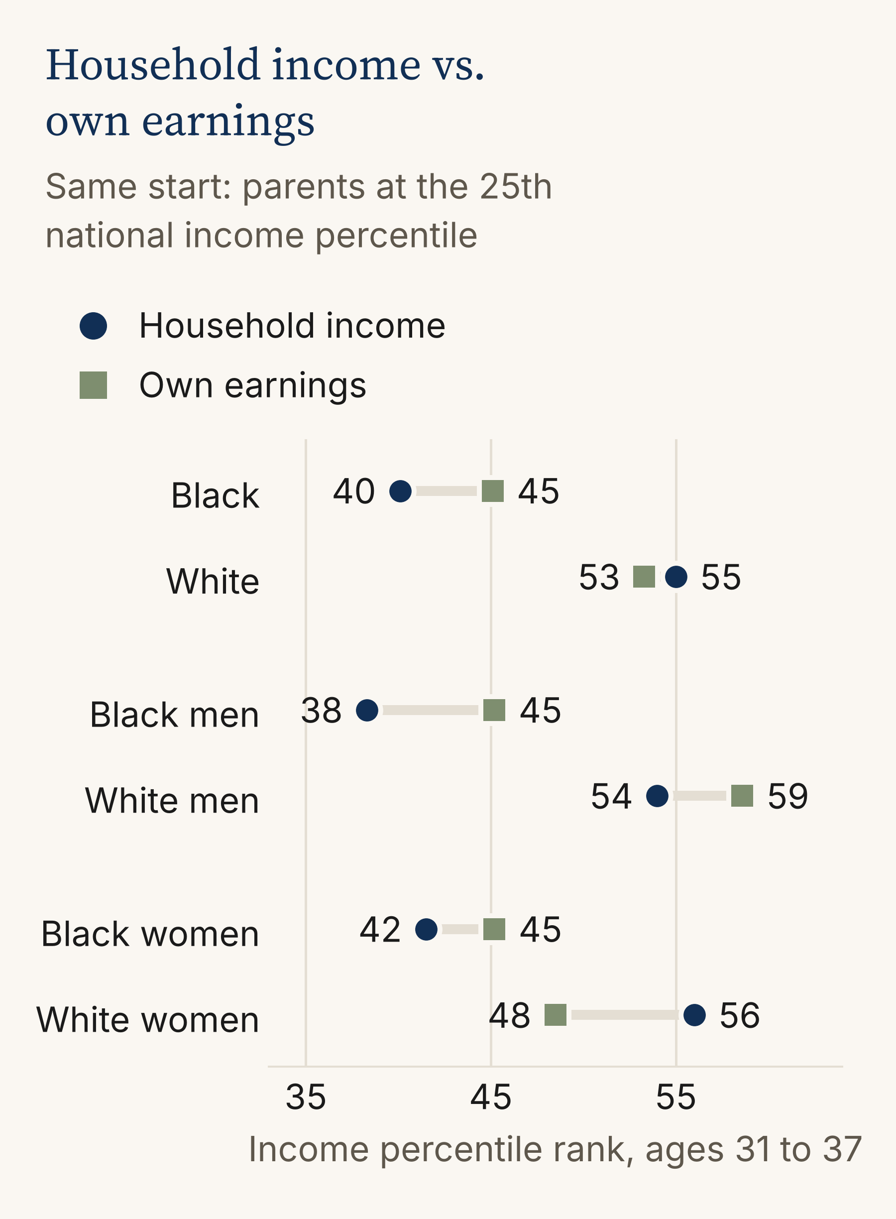
Figure 1. Household income vs. own earnings, by race and sex. Children born 1978 to 1983 who grew up in West Orange, parents at the 25th national income percentile. Household income counts a spouse's earnings; own earnings count only the person. Black men's and women's figures use 8 of 9 tracts. The women's own-earnings gap (3 points) is not statistically significant. The men's (13 points) is. Source: Opportunity Insights, Opportunity Atlas.
The household gap also has a timeline. Following the same children through their twenties, the Black-White disparity in household income was close to zero at 24, about 3 points at 26, 8 at 29, and 15 by their early-to-mid 30s. The gap in their own earnings held between 6 and 8 points from 26 on (Figure 2). Marriage moved over the same stretch. The Black-White disparity in the share married was about 6 points at 26, 17 at 29, and 20 by 2015, when 42% of the White adults from these families were married against 22% of the Black adults [1].
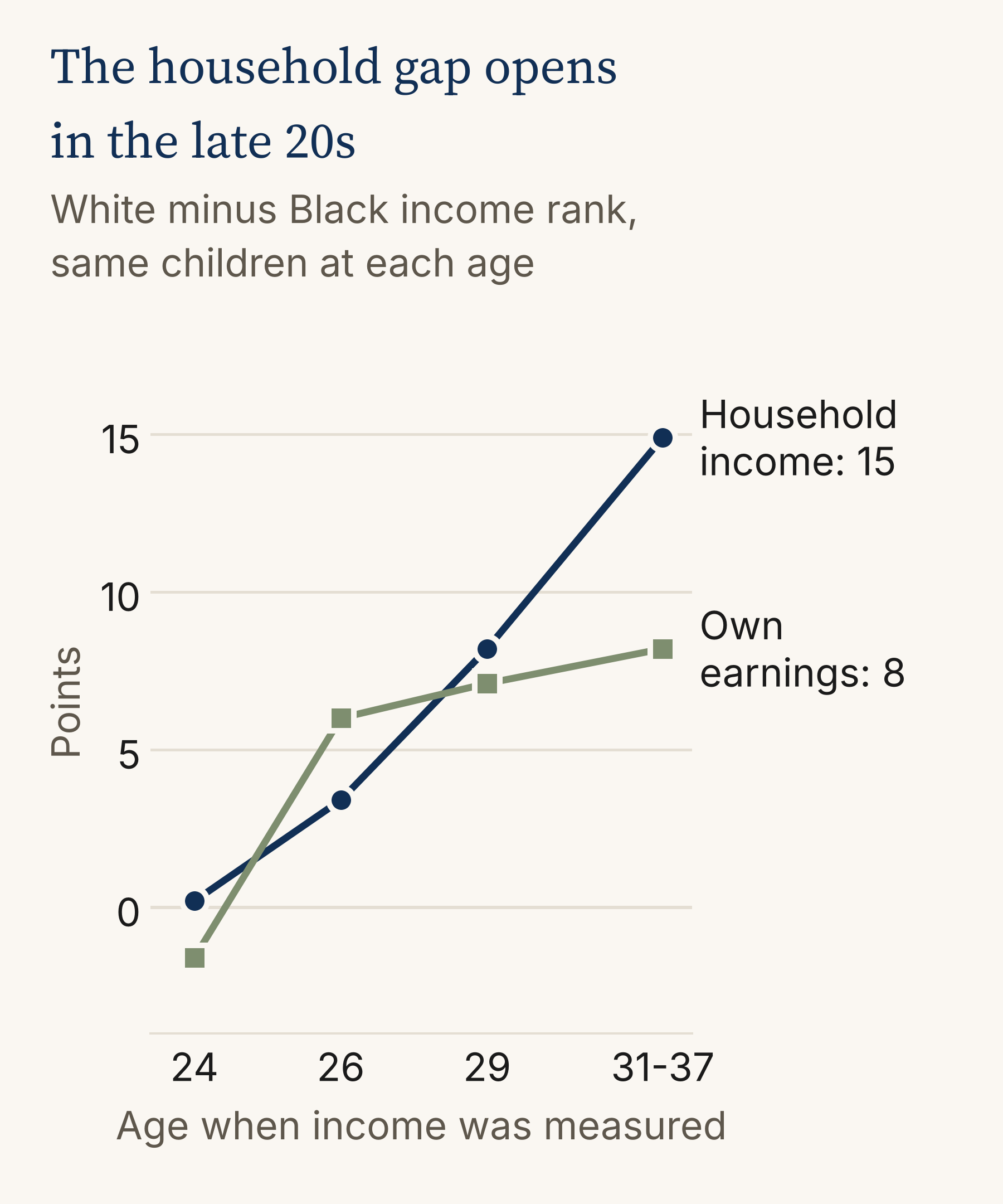
Figure 2. The Black-White gap by age. The same children measured at ages 24, 26, 29, and 31 to 37, parents at the 25th national income percentile. Each age was measured in a different calendar year (2002 to 2015). Married in 2015: 42% of White adults, 22% of Black adults. Source: Opportunity Insights, Opportunity Atlas.
I want to advocate caution with that number, because marriage statistics are often weaponized, pathologizing Black families while ignoring historical context and systemic barriers [7]. Here it matters because of how the measure is built: household income counts a spouse. A study of family structure and poverty in the South found Black-White gaps even among married parents, with poverty in married-parent households of 13.7% for Black families against 8.2% for White, and concluded that the link between family structure and racial inequality in poverty "is overstated" [7]. A second paycheck helps any household. It doesn't fix what's happening to the first one.
Back to the men, then. The pattern here matches what Chetty and colleagues found nationally: the Black-White income gap is "driven entirely by large differences in wages and employment rates between black and white men," with no such differences between Black and White women [2].
While the map can show that gap, it can't tell us why it exists. So I went looking at what research in other places has found.
Minnesota linked more than 600,000 high school graduates from the classes of 2006 through 2016 to state wage records, covering those who went on to hold a job in the state. Racial wage gaps started emerging around age 21, persisted among bachelor's degree holders, and were "much more pronounced among men than among women" [3]. Job industry appeared to play a role in part. How graduates sorted into industries gave White students, especially men, an early advantage, the report found [3].
Researchers have also tested hiring directly. In a 2001 to 2002 field experiment in Boston and Chicago, résumés with “White-sounding” names got about 50% more callbacks than the same résumés carrying “Black-sounding” names [4]. That gap showed up for male and female names alike, so it doesn't speak to why West Orange’s is a men's gap. A later audit study found that "black candidates from elite universities only do as well as white candidates from less selective universities" [5].
Over a whole career, the numbers point the same way. Nationally, among full-time, year-round workers, Black bachelor's degree holders earn a median of about $2.3 million over a career, against $2.9 million for White workers with a bachelor's degree [6].
None of that tells us what happened here. Those studies used other people, other places, and other years. The Atlas can't attribute the gap among West Orange men to hiring, to industry, or to anything else. Chetty's finding also covers employment, not just wages, and none of these studies speaks to who was working at all.
Where they lived as adults
The Atlas also records the kind of neighborhood people lived in as adults. Among children from these low-income families, 76% of White adults lived in a low-poverty tract, under 10% poverty by 2000 Census measures. For Black adults it was 44% [1]. Same starting point, a different address. In West Orange, an address carries weight even in conversation. People here sort the town by elevation, and every person Isabella Pappano interviewed for a 2025 study of the town said they had asked, or been asked, whether they were from up or down the hill [9]. How addresses in and around West Orange came to carry such different weight is its own story, one I traced in The Yellow Line.
I checked the east side
The Census figures packaged with the Atlas show poverty in our three eastern tracts doubling or tripling between 1990 and 2010, from about 7 or 8% to between 14 and 24% [1]. I wanted to know whether that showed up in the next group of kids, so I ran the comparison expecting the same trend to show up.
The Atlas has a second cohort, children born between 1984 and 1989. I compared them with the earlier group at about the same age, the late twenties (Figure 3). The east side of the town dropped 2.1 points. The rest of West Orange dropped 2.2. Essex County and the state dropped 1.7 to 1.8, and our neighbors fell anywhere from a fraction of a point to about 4 [1]. Nearly every comparison area dropped by about the same amount, which points to how the two groups were measured, in different calendar years, rather than to anything about West Orange.
The real question was whether the east side fell behind the rest of the town. While I found no clear sign of it, that conclusion comes with two limits. First, the comparison is too coarse to catch a difference smaller than about 4 or 5 points, and second, the later group can only be seen into their late twenties, before the household gap described above fully manifests.
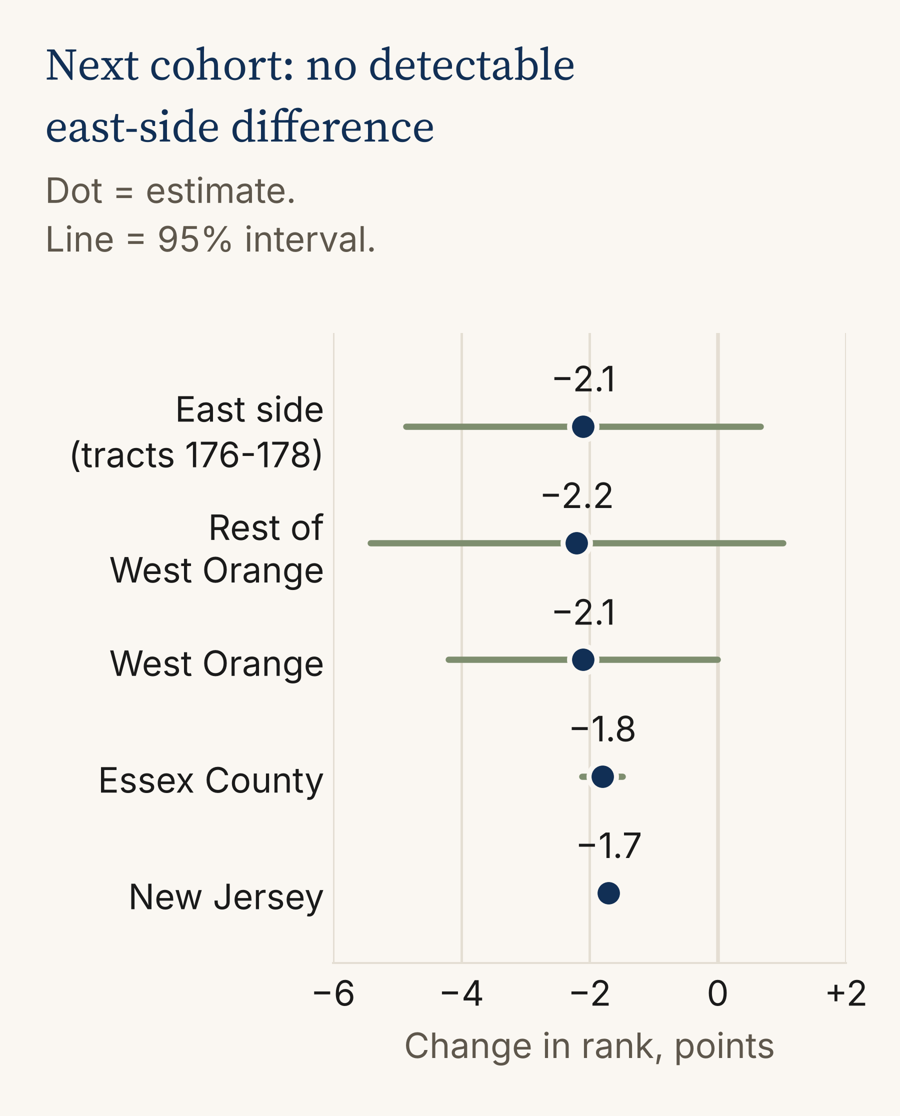
Figure 3. Change between cohorts. Children born 1984 to 1989 (ages 25 to 31) compared with children born 1978 to 1983 (average of ages 26 and 29), parents at the 25th national income percentile. The cohorts were measured in different calendar years, so the shared dip is not read as a real decline. The comparison cannot detect east-side differences smaller than about 4 to 5 points. Source: Opportunity Insights, Opportunity Atlas.
What the map can and can't tell us
The Atlas measures income, not wealth, and that matters here. A national study of young adults born in the early 1980s who went to college found the Black-White gap in student debt was largest among those whose parents had the most wealth [8]. Income rank can't see that.
So the challenge I’d put to residents, funders and curious minds alike is that one should be wary of a town average that looks healthy while hiding a 15-point gap between people who started in the same place. The council and the Board of Education could ask what local data exists on how young adults from here are doing in their mid-20s and early 30s, the years when this gap opened, and for whom. For local organizations that work with young men, that stretch of life is where, for this generation, the numbers split.
The children in this data are in their forties now. Same start. Is anyone better off?
Methods note
All West Orange figures are for children whose parents were at the 25th percentile of the national income distribution, from the Opportunity Atlas tract files [1]. They are predicted values from tract-level models, with a small amount of noise added by the Census Bureau for privacy, not counts of individual people. Town figures average West Orange's nine 2010 census tracts (173.01, 173.02, and 174 through 180), weighted by the number of children. Black men's and women's figures use 8 of the 9 tracts because one tract's estimate is suppressed. "Household income" is a person's own earnings plus a spouse's, measured in 2014 and 2015 at ages 31 to 37. "Own earnings" counts the person alone. Marriage is filing a joint or separate married tax return. Neighbor-town figures use the same method. The cohort comparison sets children born 1984 to 1989 (income at ages 25 to 31, in 2014 and 2015) against the average of the earlier cohort's incomes at ages 26 and 29 (measured 2004 to 2012). Ranks are within each birth year, but the calendar years differ, so town-level changes are not interpreted as real declines. Intervals in Figure 3 are conservative: the earlier cohort's standard error is taken as the mean of its age-26 and age-29 standard errors, since both come from the same children. The east-side comparison treats tracts 176, 177, and 178 as one group. The data cannot detect a difference between that group and the rest of town smaller than about 4 to 5 percentile points.
Reading the numbers
A few terms do a lot of work in this piece. Here is what they mean.
Percentile rank. Line up everyone born in the same year by income, lowest to highest, and split the line into 100 equal groups. Your percentile rank is the group you land in. The 47th percentile means about 47% of people your age earned less than you and about 53% earned more. Ranks are relative, so they compare people across years without worrying about inflation.
Percentile points vs. percent. A gap of 15 percentile points means two groups sit 15 places apart on that 100-step line. It does not mean one group earns 15% less. Dollar differences between ranks can be much larger or smaller depending on where on the line you are.
Parents at the 25th percentile. The Atlas compares children who started from the same place: parents who earned more than about a quarter of parents with kids the same age, roughly $27,000 a year. Holding that starting point fixed is what lets us compare groups fairly.
Household income vs. own earnings. Household income adds a spouse's earnings. Own earnings count only the person. The same adult can rank very differently on the two.
Census tract. A small area the Census Bureau draws, usually between 1,200 and 8,000 people. West Orange has nine.
Cohort. A group born in the same span of years. The main cohort here was born between 1978 and 1983. The comparison cohort was born between 1984 and 1989.
Predicted value. The Atlas doesn't report a simple average of real people. It fits a model within each tract and reports what that model predicts for a child whose parents were at the 25th percentile. The Census Bureau also adds a small amount of random noise to protect privacy.
Standard error. Every estimate from a sample comes with some uncertainty. The standard error measures how much an estimate would likely bounce around if you could repeat the measurement with a different set of people. Smaller is more precise. Estimates built on many people, like the whole state, have small standard errors. Estimates built on a few hundred people, like one West Orange tract, have larger ones.
95% interval. A range built from the standard error, roughly the estimate plus or minus two standard errors. If the measurement were repeated many times, ranges built this way would capture the true value about 95% of the time. In Figure 3, the lines around each dot are these intervals.
Statistically significant. A difference is called significant when it is large compared with its uncertainty, too large to be easily explained by noise. The 3-point gap between Black and White women's own earnings is not. The 13-point gap between men is.
Detection limit. The smallest difference a comparison could reliably pick up. For the east-side check, a gap smaller than about 4 or 5 points could be there without the data being able to show it. "No sign of a difference" is not the same as "no difference."
References
Chetty, R., Friedman, J. N., Hendren, N., Jones, M. R., & Porter, S. R. (2018). The Opportunity Atlas: Mapping the childhood roots of social mobility (NBER Working Paper No. 25147). National Bureau of Economic Research. Data: Opportunity Insights, Opportunity Atlas tract-level outcomes, early (1978 to 1983) and late (1984 to 1989) birth cohorts, and tract covariates. https://opportunityinsights.org/data/
Chetty, R., Hendren, N., Jones, M. R., & Porter, S. R. (2020). Race and economic opportunity in the United States: An intergenerational perspective. Quarterly Journal of Economics, 135(2), 711-783.
Leibert, A. (2021, March). How the deck is stacked: Racial and ethnic disparities in earnings following high school graduation in Minnesota. Minnesota Department of Employment and Economic Development. https://mn.gov/deed/newscenter/publications/trends/march-2021/deck-is-stacked.jsp
Bertrand, M., & Mullainathan, S. (2004). Are Emily and Greg more employable than Lakisha and Jamal? A field experiment on labor market discrimination. American Economic Review, 94(4), 991-1013. https://doi.org/10.1257/0002828042002561
Gaddis, S. M. (2015). Discrimination in the credential society: An audit study of race and college selectivity in the labor market. Social Forces, 93(4), 1451-1479. https://doi.org/10.1093/sf/sou111
Carnevale, A. P., Cheah, B., & Wenzinger, E. (2021). The college payoff: More education doesn't always mean more earnings. Georgetown University Center on Education and the Workforce. https://cew.georgetown.edu/collegepayoff2021
Baker, R. S., & O'Connell, H. A. (2022). Structural racism, family structure, and Black-White inequality: The differential impact of the legacy of slavery on poverty among single mother and married parent households. Journal of Marriage and Family, 84(5), 1341-1365. https://doi.org/10.1111/jomf.12837
Addo, F. R., Houle, J. N., & Simon, D. (2016). Young, Black, and (still) in the red: Parental wealth, race, and student loan debt. Race and Social Problems, 8(1), 64-76. https://doi.org/10.1007/s12552-016-9162-0
Pappano, I. (2025). Settlement and linguistic patterns of West Orange, New Jersey. TCNJ Journal of Student Scholarship, 27.